Note
Click here to download the full example code
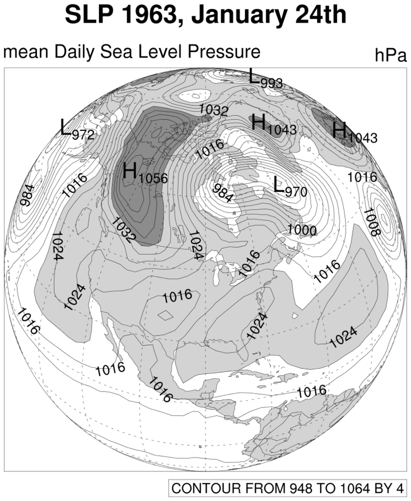
NCL_sat_2.py
- This script illustrates the following concepts:
Converting float data into short data
Drawing filled contours over a satellite map
Explicitly setting contour fill colors
Finding local high pressure values
- See following URLs to see the reproduced NCL plot & script:
Original NCL script: https://www.ncl.ucar.edu/Applications/Scripts/sat_2.ncl
Original NCL plot: https://www.ncl.ucar.edu/Applications/Images/sat_2_lg.png
Import packages:
import xarray as xr
import cartopy.crs as ccrs
import cartopy.feature as cfeature
import numpy as np
from sklearn.cluster import DBSCAN
import matplotlib.pyplot as plt
from matplotlib import colors
import matplotlib.ticker as mticker
import warnings

import geocat.datafiles as gdf
import geocat.viz.util as gvutil
Read in data:
# Open a netCDF data file using xarray default engine and
# load the data into xarrays
ds = xr.open_dataset(gdf.get("netcdf_files/slp.1963.nc"), decode_times=False)

# Get data from the 21st timestep
pressure = ds.slp[21, :, :]

# Translate float values to short values
pressure = pressure.astype('float32')

# Convert Pa to hPa data
pressure = pressure * 0.01

# Fix the artifact of not-shown-data around 0 and 360-degree longitudes
wrap_pressure = gvutil.xr_add_cyclic_longitudes(pressure, "lon")
def findLocalExtrema(da, highVal=0, lowVal=1000, eType='Low'):
    """
    Utility function to find local low/high field variable coordinates on a contour map. To classify as a local high, the data
    point must be greater than highVal, and to classify as a local low, the data point must be less than lowVal.
    Args:
        da: (:class:`xarray.DataArray`):
            Xarray data array containing the lat, lon, and field variable (ex. pressure) data values
        highVal (:class:`int`):
            Data value that the local high must be greater than to qualify as a "local high" location.
            Default highVal is 0.
        lowVal (:class:`int`):
            Data value that the local low must be less than to qualify as a "local low" location.
            Default lowVal is 1000.
        eType (:class:`str`):
            'Low' or 'High'
            Determines which extrema are being found- minimum or maximum, respectively.
            Default eType is 'Low'.
    Returns:
        clusterExtremas (:class:`list`):
            List of coordinate tuples in GPS form (lon in degrees, lat in degrees)
            that specify local low/high locations
    """

    # Create a 2D array of coordinates in the same shape as the field variable data
    # so each coordinate is easily mappable to a data value
    # ex:
    # (1, 1), (2, 1), (3, 1)
    # (1, 2)................
    # (1, 3)................
    lons, lats = np.meshgrid(np.array(da.lon), np.array(da.lat))
    coordarr = np.dstack((lons, lats))

    # Find all zeroes that also qualify as low or high values
    extremacoords = []

    if eType == 'Low':
        coordlist = np.argwhere(da.data < lowVal)
        extremacoords = [tuple(coordarr[x[0]][x[1]]) for x in coordlist]
    if eType == 'High':
        coordlist = np.argwhere(da.data > highVal)
        extremacoords = [tuple(coordarr[x[0]][x[1]]) for x in coordlist]

    if extremacoords == []:
        if eType == 'Low':
            warnings.warn(
                'No local extrema with data value less than given lowVal')
            return []
        if eType == 'High':
            warnings.warn(
                'No local extrema with data value greater than given highVal')
            return []

    # Clean up noisy data to find actual extrema

    # Use Density-based spatial clustering of applications with noise
    # to cluster and label coordinates
    db = DBSCAN(eps=10, min_samples=1)
    new = db.fit(extremacoords)
    labels = new.labels_

    # Create an dictionary of values with key being coordinate
    # and value being cluster label.
    coordsAndLabels = {label: [] for label in labels}
    for label, coord in zip(labels, extremacoords):
        coordsAndLabels[label].append(coord)

    # Initialize array of coordinates to be returned
    clusterExtremas = []

    # Iterate through the coordinates in each cluster
    for key in coordsAndLabels:

        # Create array to hold all the field variable values for that cluster
        datavals = []
        for coord in coordsAndLabels[key]:

            # Find pressure data at that coordinate
            cond = np.logical_and(coordarr[:, :, 0] == coord[0],
                                  coordarr[:, :, 1] == coord[1])
            x, y = np.where(cond)
            datavals.append(da.data[x[0]][y[0]])

        # Find the index of the smallest/greatest field variable value of each cluster
        if eType == 'Low':
            index = np.argmin(np.array(datavals))
        if eType == 'High':
            index = np.argmax(np.array(datavals))

        # Append the coordinate corresponding to that index to the array to be returned
        clusterExtremas.append(
            (coordsAndLabels[key][index][0], coordsAndLabels[key][index][1]))

    return clusterExtremas
def plotCLabels(ax,
                contours,
                transform,
                proj,
                clabel_locations=[],
                fontsize=12,
                whitebbox=False,
                horizontal=False):
    """
    Utility function to plot contour labels by passing in a coordinate to the clabel function.
    This allows the user to specify the exact locations of the labels, rather than having matplotlib
    plot them automatically.
    This function is exemplified in the python version of https://www.ncl.ucar.edu/Applications/Images/sat_1_lg.png
    Args:
        ax (:class:`matplotlib.pyplot.axis`):
            Axis containing the contour set.
        contours (:class:`cartopy.mpl.contour.GeoContourSet`):
            Contour set that is being labeled.
        transform (:class:`cartopy._crs`):
            Instance of CRS that represents the source coordinate system of coordinates.
            (ex. ccrs.Geodetic()).
        proj (:class:`cartopy.crs`):
            Projection 'ax' is defined by.
            This is the instance of CRS that the coordinates will be transformed to.
        clabel_locations (:class:`list`):
            List of coordinate tuples in GPS form (lon in degrees, lat in degrees)
            that specify where the contours with regular field variable values should be plotted.
        fontsize (:class:`int`):
            Font size of contour labels.
        whitebbox (:class:`bool`):
            Setting this to "True" will cause all labels to be plotted with white backgrounds
        horizontal (:class:`bool`):
            Setting this to "True" will cause the contour labels to be horizontal.
    Returns:
        cLabels (:class:`list`):
            List of text instances of all contour labels
    """

    # Initialize empty array that will be filled with contour label text objects and returned
    cLabels = []

    # Plot any regular contour levels
    if clabel_locations != []:
        clevelpoints = proj.transform_points(
            transform, np.array([x[0] for x in clabel_locations]),
            np.array([x[1] for x in clabel_locations]))
        transformed_locations = [(x[0], x[1]) for x in clevelpoints]
        ax.clabel(contours,
                  manual=transformed_locations,
                  inline=True,
                  fontsize=fontsize,
                  colors='black',
                  fmt="%.0f")
        [cLabels.append(txt) for txt in contours.labelTexts]

        if horizontal is True:
            [txt.set_rotation('horizontal') for txt in contours.labelTexts]

    if whitebbox is True:
        [
            txt.set_bbox(dict(facecolor='white', edgecolor='none', pad=2))
            for txt in cLabels
        ]

    return cLabels
def plotELabels(transform,
                proj,
                da,
                clabel_locations=[],
                label='L',
                fontsize=22,
                whitebbox=False,
                horizontal=True):
    """
    Utility function to plot contour labels. High/Low contour labels will be plotted using text boxes for more accurate label values
    and placement.
    This function is exemplified in the python version of https://www.ncl.ucar.edu/Applications/Images/sat_1_lg.png
    Args:
        da: (:class:`xarray.DataArray`):
            Xarray data array containing the lat, lon, and field variable data values.
        transform (:class:`cartopy._crs`):
            Instance of CRS that represents the source coordinate system of coordinates.
            (ex. ccrs.Geodetic()).
        proj (:class:`cartopy.crs`):
            Projection 'ax' is defined by.
            This is the instance of CRS that the coordinates will be transformed to.
        clabel_locations (:class:`list`):
            List of coordinate tuples in GPS form (lon in degrees, lat in degrees)
            that specify where the contour labels should be plotted.
        label (:class:`str`):
            ex. 'L' or 'H'
            The data value will be plotted as a subscript of this label.
        fontsize (:class:`int`):
            Font size of regular contour labels.
        horizontal (:class:`bool`):
            Setting this to "True" will cause the contour labels to be horizontal.
        whitebbox (:class:`bool`):
            Setting this to "True" will cause all labels to be plotted with white backgrounds
    Returns:
        extremaLabels (:class:`list`):
            List of text instances of all contour labels
    """

    # Create array of coordinates in the same shape as field variable data
    # so each coordinate can be easily mapped to its data value.
    # ex:
    # (1, 1), (2, 1), (3, 1)
    # (1, 2)................
    # (1, 3)................
    lons, lats = np.meshgrid(np.array(da.lon), np.array(da.lat))
    coordarr = np.dstack((lons, lats))

    # Initialize empty array that will be filled with contour label text objects and returned
    extremaLabels = []

    # Plot any low contour levels
    clabel_points = proj.transform_points(
        transform, np.array([x[0] for x in clabel_locations]),
        np.array([x[1] for x in clabel_locations]))
    transformed_locations = [(x[0], x[1]) for x in clabel_points]

    for x in range(len(transformed_locations)):

        try:
            # Find field variable data at that coordinate
            coord = clabel_locations[x]
            cond = np.logical_and(coordarr[:, :, 0] == coord[0],
                                  coordarr[:, :, 1] == coord[1])
            z, y = np.where(cond)
            p = int(round(da.data[z[0]][y[0]]))

            lab = plt.text(transformed_locations[x][0],
                           transformed_locations[x][1],
                           label + "$_{" + str(p) + "}$",
                           fontsize=fontsize,
                           horizontalalignment='center',
                           verticalalignment='center')

            if horizontal is True:
                lab.set_rotation('horizontal')

            extremaLabels.append(lab)

        except Exception as E:
            print(E)
            continue

    if whitebbox is True:
        [
            txt.set_bbox(dict(facecolor='white', edgecolor='none', pad=2))
            for txt in extremaLabels
        ]

    return extremaLabels
# Create plot

# Set figure size
fig = plt.figure(figsize=(8, 8))

# Set global axes with an orthographic projection
proj = ccrs.Orthographic(central_longitude=270, central_latitude=45)
ax = plt.axes(projection=proj)
ax.set_global()

# Add land, coastlines, and ocean features
ax.add_feature(cfeature.LAND, facecolor='lightgray', zorder=1)
ax.add_feature(cfeature.COASTLINE, linewidth=.3, zorder=2)
ax.add_feature(cfeature.OCEAN, facecolor='white')
ax.add_feature(cfeature.BORDERS, linewidth=.3)
ax.add_feature(cfeature.LAKES, facecolor='white', edgecolor='black', linewidth=.3)

# Create color map
colorvalues = [1020, 1036, 1500]
cmap = colors.ListedColormap(['None', 'lightgray', 'dimgrey'])
norm = colors.BoundaryNorm(colorvalues, 2)

# Plot contour data
p = wrap_pressure.plot.contourf(ax=ax,
                                zorder=2,
                                transform=ccrs.PlateCarree(),
                                levels=30,
                                cmap=cmap,
                                norm=norm,
                                add_labels=False,
                                add_colorbar=False)

p = wrap_pressure.plot.contour(ax=ax,
                               transform=ccrs.PlateCarree(),
                               linewidths=0.3,
                               levels=30,
                               cmap='black',
                               add_labels=False)

# low pressure contour levels- these will be plotted
# as a subscript to an 'L' symbol.
lowClevels = findLocalExtrema(pressure, lowVal=995, eType='Low')
highClevels = findLocalExtrema(pressure, highVal=1042, eType='High')

# Label regular contours with automatic matplotlib labeling
# Specify the levels to label every other contour level
ax.clabel(p,
          levels=np.arange(956, 1064, 8),
          inline=True,
          fontsize=12,
          colors='black',
          fmt="%.0f")

# Label low and high contours
plotELabels(ccrs.Geodetic(),
            proj,
            wrap_pressure,
            clabel_locations=lowClevels,
            label='L')
plotELabels(ccrs.Geodetic(),
            proj,
            wrap_pressure,
            clabel_locations=highClevels,
            label='H')

# Use gvutil function to set title and subtitles
gvutil.set_titles_and_labels(ax,
                             maintitle=r"$\bf{SLP}$" + " " + r"$\bf{1963,}$" +
                             " " + r"$\bf{January}$" + " " + r"$\bf{24th}$",
                             maintitlefontsize=20,
                             lefttitle="mean Daily Sea Level Pressure",
                             lefttitlefontsize=16,
                             righttitle="hPa",
                             righttitlefontsize=16)

# Set characteristics of text box
props = dict(facecolor='white', edgecolor='black', alpha=0.5)

# Place text box
ax.text(0.40,
        -0.1,
        'CONTOUR FROM 948 TO 1064 BY 4',
        transform=ax.transAxes,
        fontsize=16,
        bbox=props)

# Add gridlines to axis
gl = ax.gridlines(color='gray', linestyle='--')
gl.xlocator = mticker.FixedLocator(np.arange(-180, 180, 20))
gl.ylocator = mticker.FixedLocator(np.arange(-90, 90, 20))

# Make layout tight
plt.tight_layout()

plt.show()

Total running time of the script: ( 0 minutes 1.642 seconds)