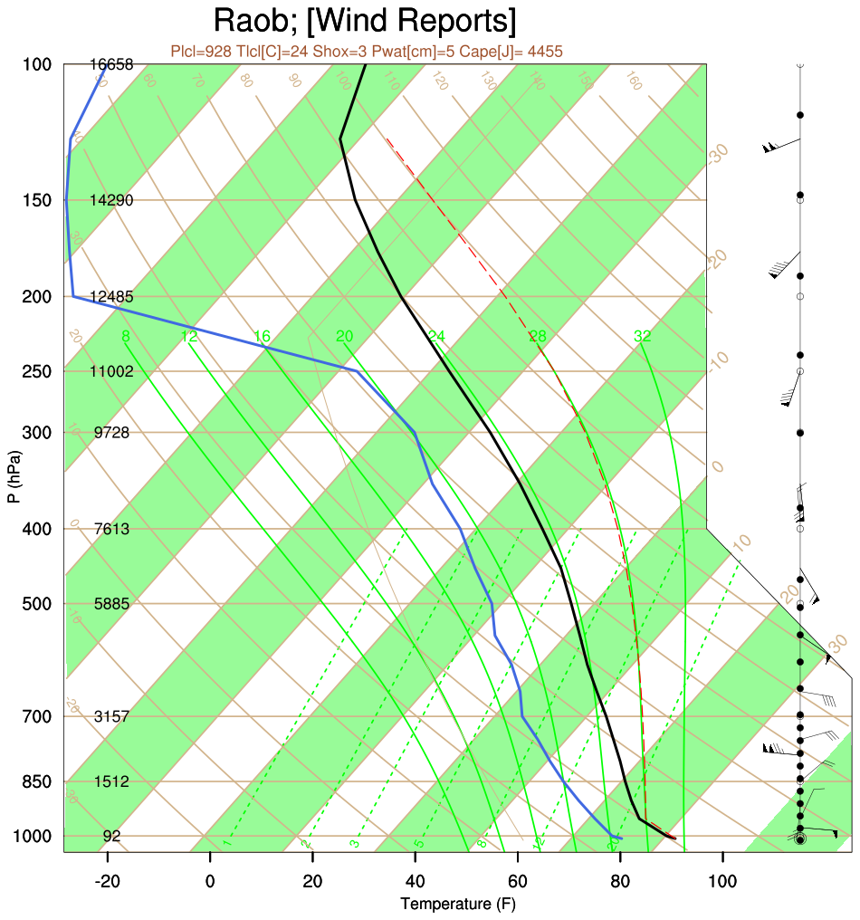
NCL_skewt_2_2.py

This script illustrates the following concepts:

• Customizing the background of a Skew-T plot

• Plotting temperature, dewpoint, and wind data on a Skew-T plot

See following URLs to see the reproduced NCL plot & script:

• Original NCL script: https://www.ncl.ucar.edu/Applications/Scripts/skewt_2.ncl

• Original NCL plots: https://www.ncl.ucar.edu/Applications/Images/skewt_2_2_lg.png

Note:

Currently functions to calculate CAPE, precipitable water, the showalter index, the pressure of the LCL, and the temperature of the LCL do not exist in geocat-comp. An issue has been opened on the geocat-comp GitHub. The subtitle with those values will be added at a later date once that issue has been closed.

Import packages:

import matplotlib.pyplot as plt
import matplotlib.lines as mlines
import numpy as np
import pandas as pd
from metpy.plots import SkewT
from metpy.units import units
import metpy.calc as mpcalc

import geocat.viz.util as gvutil
import geocat.datafiles as gdf

Read in data:

# Open a netCDF data file using xarray default engine and load the data into xarrays
ds = pd.read_csv(gdf.get('ascii_files/sounding.testdata'), delimiter='\\s+', header=None)

# Extract the data
p = ds[1].values*units.hPa   # Pressure [mb/hPa]
tc = (ds[5].values + 2)*units.degC  # Temperature [C]
tdc = ds[9].values*units.degC  # Dew pt temp  [C]

# Create dummy wind data
wspd = np.linspace(0, 150, len(p))*units.knots    # Wind speed   [knots or m/s]
wdir = np.linspace(0, 360, len(p))*units.degrees    # Meteorological wind dir
u, v = mpcalc.wind_components(wspd, wdir)   # Calculate wind components

Plot:

# Note that MetPy forces the x axis scale to be in Celsius and the y axis
# scale to be in hectoPascals. Once data is plotted, then the axes labels are
# automatically added
fig = plt.figure(figsize=(12, 12))

# The rotation keyword changes how skewed the temperature lines are. MetPy has
# a default skew of 30 degrees
skew = SkewT(fig, rotation=45)
ax = skew.ax

# Plot temperature and dew point
skew.plot(p, tc, color='black')
skew.plot(p, tdc, color='blue')

# Draw parcel path
parcel_prof = mpcalc.parcel_profile(p, tc[0], tdc[0]).to('degC')
skew.plot(p, parcel_prof, color='red', linestyle='--')
u = np.where(p>=100*units.hPa, u, np.nan)
v = np.where(p>=100*units.hPa, v, np.nan)
p = np.where(p>=100*units.hPa, p, np.nan)

# Add wind barbs
skew.plot_barbs(p=p[::2],
                u=u[::2],
                v=v[::2],
                xloc=1.05,
                fill_empty=True,
                sizes=dict(emptybarb=0.075, width=0.1, height=0.2))

# Draw line underneath wind barbs
line = mlines.Line2D([1.05, 1.05], [0, 1],
                     color='gray',
                     linewidth=0.5,
                     transform=ax.transAxes,
                     clip_on=False,
                     zorder=1)
ax.add_line(line)

# Shade every other section between isotherms
x1 = np.linspace(-100, 40, 8)  # The starting x values for the shaded regions
x2 = np.linspace(-90, 50, 8)  # The ending x values for the shaded regions
y = [1050, 100]  # The range of y values that the shades regions should cover
for i in range(0, 8):
    skew.shade_area(y=y,
                    x1=x1[i],
                    x2=x2[i],
                    color='limegreen',
                    alpha=0.25,
                    zorder=1)

# Choose starting temperatures in Kelvin for the dry adiabats
t0 = units.K * np.arange(243.15, 444.15, 10)
skew.plot_dry_adiabats(t0=t0, linestyles='solid', colors='tan', linewidths=1.5)

# Choose starting temperatures in Kelvin for the moist adiabats
t0 = units.K * np.arange(281.15, 306.15, 4)
skew.plot_moist_adiabats(t0=t0,
                         linestyles='solid',
                         colors='lime',
                         linewidth=1.5)

# Choose mixing ratios
w = np.array([0.001, 0.002, 0.003, 0.005, 0.008, 0.012, 0.020]).reshape(-1, 1)

# Choose the range of pressures that the mixing ratio lines are drawn over
p_levs = units.hPa * np.linspace(1000, 400, 7)

# Plot mixing ratio lines
skew.plot_mixing_lines(w=w,
                       p=p_levs,
                       linestyle='dashed',
                       colors='lime',
                       linewidths=1)

# Use geocat.viz utility functions to set axes limits and ticks
gvutil.set_axes_limits_and_ticks(
    ax=ax,
    xlim=[-32, 38],
    yticks=[1000, 850, 700, 500, 400, 300, 250, 200, 150, 100])

# Use geocat.viz utility function to change the look of ticks and ticklabels
gvutil.add_major_minor_ticks(ax=ax,
                             x_minor_per_major=1,
                             y_minor_per_major=1,
                             labelsize=14)
# The utility function draws tickmarks all around the plot. We only need ticks
# on the left and bottom edges
ax.tick_params('both', which='both', top=False, right=False)

# Use geocat.viz utility functions to add a main title
gvutil.set_titles_and_labels(ax=ax,
                             maintitle="Raob; [Wind Reports]",
                             maintitlefontsize=22,
                             xlabel='Temperature (C)',
                             ylabel='P (hPa)',
                             labelfontsize=14)

# Change the style of the gridlines
plt.grid(True,
         which='major',
         axis='both',
         color='tan',
         linewidth=1.5,
         alpha=0.5)

plt.show()